Week08 Day39

mini-code

print(0.1 + 0.2, 0.1 + 0.2 == 0.3) # 0.3 False
val = 0
for _ in range(10):
  val += 0.1
print(val, val == 1.0) # 0.999999 False

이번 mini-code는 정밀도(precision)에 대한 것이다.
컴퓨터는 모든 수를 2진수로 나타내는데 0.1이나 0.2는 유한소수이지만 2진수로 나타내면 무한소수가 된다.
고정된 길이의 비트를 사용하기 때문에 소수를 정확하게 표현하지 못할 수 있다.
실제로 0.1과 0.2를 소수점 30자리까지 출력해보면 다음과 같이 부정확하다는 것을 알 수 있다.

a = 0.1
b = 0.2
print(f"{a.30f}") # 0.100000000000000005551115123126
print(f"{b.30f}") # 0.200000000000000011102230246252

이전에 고정 소수점과 부동 소수점에 대해 정리했다.

아래 예시처럼 모든 실수가 오차를 갖는건 아니다.

val2 = 0
for _ in range(64):
  val2 += 1 / 64
print(val2, val2 == 1.0) # 1.0 True

위 예시처럼 분자는 integer, 분모가 2의 거듭제곱일 때 오차없이 표현할 수 있다.
그러면 python에서 두 실수가 같음을 어떻게 판단할까?
이 글을 참고했다.

import sys
import math
a = 0.1 + 0.2
b = 0.3
print(math.fabs(a - b) <= sys.float_info.epsilon) # True
print(math.isclose(a, b)) # True

math.fabs는 절대값을 반환한다.

여기서 sys.float_info.epsilon에 저장된 값을 머신 엡실론(machine epsilon)이라고 부르는데, 어떤 실수를 가장 가까운 부동소수점 실수로 반올림했을 때 상대 오차는 항상 머신 엡실론 이하입니다. 즉, 머신 엡실론은 반올림 오차의 상한값이며 연산한 값과 비교할 값의 차이가 머신 엡실론보다 작거나 같다면 두 실수는 같은 값이라 할 수 있습니다.

FPU(Floating Point Unit)

이 부분은 이 글을 참고하여 작성했다.

Stands for “Floating Point Unit.” An FPU is a processor or part of a processor that performs floating point calculations. While early FPUs were standalone processors, most are now integrated inside a computer’s CPU.

FPU는 floating point unit의 약자이고 floating point 계산을 수행하는 프로세서이다.
이전에는 CPU 밖에 있었는데 요즘은 속도 향상을 위해 내부에 위치해 있다.
사실 CPU가 integer, floating point 둘 다 계산할 수 있지만 비효율적이다.
둘의 연산이 상당히 다르기 때문이다.
그래서 FPU를 사용하면 non-integer 연산을 효율적으로 할 수 있다.

Making Neural Nets Work With Low Precision

이 글 읽고 정리하기…

quantization

이 부분은 여기를 참고해서 작성했다.
양자화(quantization)은 floating-point precision보다 더 낮은 bit-widths에서 계산하고 tensor를 저장하는 기술이다.
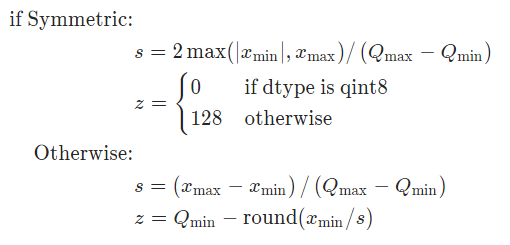
floating-point와 fixed-point precision 사이를 변환하는 식은 다음과 같다.
$Q(x,\ scale,\ zero-point) = round(\frac{x}{scale} + zero-point)$ 여기서 $x$ 는 floating-point input, $Q$ 는 양자화 output이다.
수식에 대한 자세한 설명은 이 곳을 참조한다.

pytorch에서 양자화는 float32를 int8로 변환을 지원하며 다음과 같은 특성이 있다.

모델 사이즈 감소
memory bandwidth 요구 감소
on-device int8 계산은 float32과 비교하여 더 빠르다.
양자화는 주로 inference를 빠르게 하는 기술이다.
int8로 float32를 근사하는 것이라서 약간 accuracy의 감소가 있다.

양자화는 크게 3가지로 분류할 수 있다.

Dynamic quantization
Post-training static quantization
Quantization aware training

양자화는 제한된 operator들을 갖는다.
이런 operator들은 모델이 동작하는 하드웨어에 따라 다르다.
예를 들어 x86 and ARM에서는 operator들은 오직 CPU로만 inference를 진행한다.
그러나 quantization aware training은 full floating-point를 사용하며 CPU 혹은 GPU 둘 중 하나를 사용할 수 있다.
이 방법은 post-training static 혹은 dynamic quantization의 성능이 좋지 못하면 사용된다.

양자화 방법들을 좀 더 알아보자.
QUANTIZATION와 Introduction to Quantization on PyTorch를 참조했다.

Dynamic quantization

이 부분은 이 글을 참조했다.
Dynamic quantization (weights quantized with activations read/stored in floating point and quantized for compute.)

This is the simplest to apply form of quantization where the weights are quantized ahead of time but the activations are dynamically quantized during inference.
This is used for situations where the model execution time is dominated by loading weights from memory rather than computing the matrix multiplications.
This is true for for LSTM and Transformer type models with small batch size.

DQ(Dynamic quantization)는 inference할 때 activations을 양자화하고 학습할 때는 다시 floating-point로 저장한다.
이 방법은 양자화의 가장 간단한 형태이고 행렬 곱셈보다 오히려 메모리에서 weight를 불러와서 모델 실행시간이 길 때 사용된다.
이 경우는 작은 batch size를 가진 LSTM과 Transformer 타입의 모델에 해당된다.

The key idea with dynamic quantization is that we are going to determine the scale factor for activations dynamically based on the data range observed at runtime.
This ensures that the scale factor is “tuned” so that as much signal as possible about each observed dataset is preserved.

DQ의 주된 아이디어는 runtime에서 관찰된 데이터 범위에 기반하여 동적으로 activations에 대한 scale factor를 결정하는 것이다.
scale factor가 tuned 되어 관찰된 데이터에 대해 가능한 많은 signal가 보존됨을 보장한다.

import torch

# define a floating point model
class M(torch.nn.Module):
    def __init__(self):
        super(M, self).__init__()
        self.fc = torch.nn.Linear(3, 5, False)

    def forward(self, x):
        x = self.fc(x)
        return x

# create a model instance
model_fp32 = M()
# create a quantized model instance
model_int8 = torch.quantization.quantize_dynamic(
    model_fp32,  # the original model
    {torch.nn.Linear},  # a set of layers to dynamically quantize
    dtype=torch.qint8)  # the target dtype for quantized weights

# run the model
input_fp32 = torch.randn(2, 3)
res = model_int8(input_fp32)

DQ 예시이다.
실제로 어떻게 weight를 quantization하는지 알아내는데 엄청 고생했다.
MinMaxObserver를 사용하고 torch.per_tensor_symmetric scheme을 사용한다.
¹
엄청 고생한 이유는 scale factor를 구할 때 (Tensor의 최대값 - 최소값) / 255 라고 생각했는데 최대값 / (255 / 2)로 계산한다.
최대값과 최소값이 같으면 scale factor와 zero_point는 1, 0으로 정해진다.

Post-training static quantization

Static quantization (weights quantized, activations quantized, calibration required post training)

Static quantization quantizes the weights and activations of the model.
It fuses activations into preceding layers where possible.
It requires calibration with a representative dataset to determine optimal quantization parameters for activations.
Post Training Quantization is typically used when both memory bandwidth and compute savings are important with CNNs being a typical use case.
Static quantization is also known as Post Training Quantization or PTQ.

PTQ(Post-training static quantization)는 학습 후 weight와 activation을 양자화한다.
activations에 대한 최적의 양자화 parameter를 결정하기 위해 representative dataset과 함께 미세한 조정이 필요하다.
PTQ는 메모리 대역폭과 계산 절약이 둘 다 중요할 때 사용되며 CNN이 대표적인 예시이다.

Quantization aware training

Quantization aware training (weights quantized, activations quantized, quantization numerics modeled during training)

Quantization Aware Training models the effects of quantization during training allowing for higher accuracy compared to other quantization methods.
During training, all calculations are done in floating point, with fake_quant modules modeling the effects of quantization by clamping and rounding to simulate the effects of INT8.
After model conversion, weights and activations are quantized, and activations are fused into the preceding layer where possible.
It is commonly used with CNNs and yields a higher accuracy compared to static quantization.
Quantization Aware Training is also known as QAT.

QAT(Quantization aware training)는 weight, activation을 양자화하고 학습 중에도 양자화한다.
이 방법은 다른 양자화 방법과 비교하여 학습 중 높은 정확도를 보이며 양자화 효과를 모델링한다.
학습하는 동안에 모든 계산들은 floating-point로 수행되며, fake_quant는 int8의 효과를 시뮬레이션하기 위해 clamping과 반올림하여 양자화 효과를 모델링한다.
모델 변환 후 weight과 activations는 양자화되고 activations은 가능하다면 이전 layer에 합쳐진다.
이 방법은 주로 CNN과 함께 사용되며 PTQ와 비교하여 더 높은 정확도를 보인다.

쉽게 말하면 QAT는 학습 중 forward와 backward 동안 모든 weights와 activations을 fake quantization한다.
float values는 int8을 흉내내기 위해 반올림하지만 모든 계산은 floating-point으로 수행된다.
학습 중 모든 weights 조정은 모델이 궁극적으로 양자화될 것이라는 사실을 인식하며 이루어진다.
그러므로 양자화 후 이 방법은 다른 두 방법보다 대개 높은 정확도를 가진다.

comparison

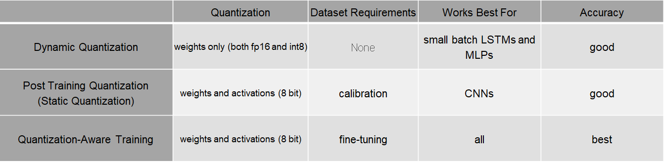
위 세가지 방법을 비교했다.
²
아직 공부가 부족하여 왜 위와 같은 특성이 나타나는지 모르겠다.
나중에 추가할 예정이다…

toy-code

사용한 모델은 ResNet이며 mnist를 학습했으며 DQ를 사용했다.

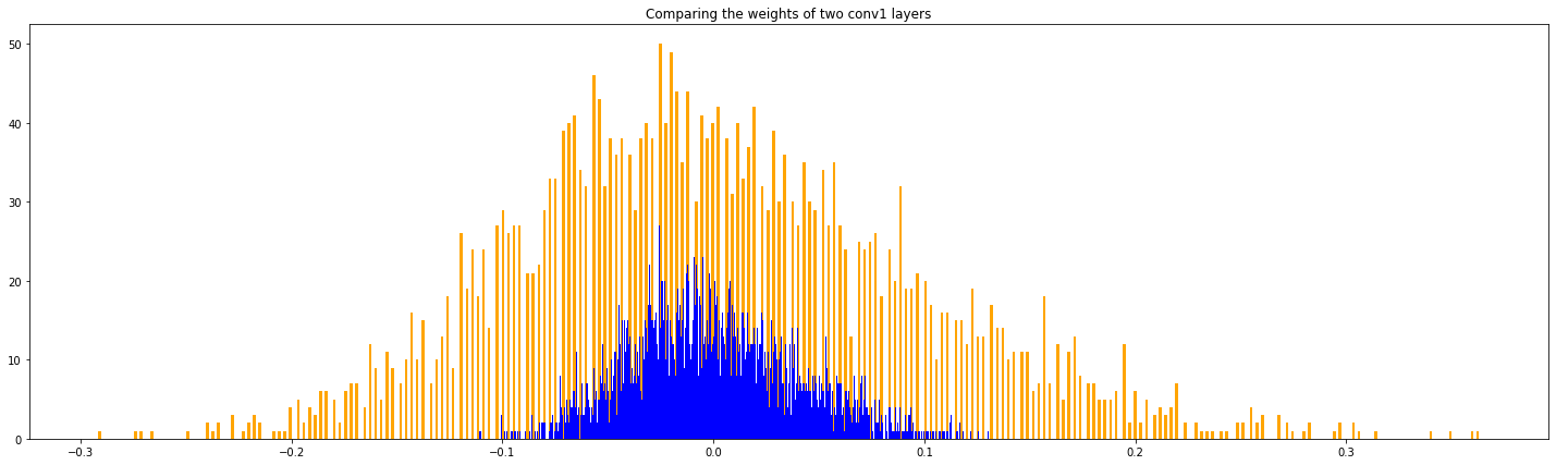
위 그림은 첫번째 convolutional layer의 weight의 histogram을 그려봤다.
파란색은 original weight에 대한 분포이며 0 주변에 몰려있다.
오렌지색은 quantized weight를 dequantization한 weight에 대한 분포이며 0을 중심으로 좌우로 퍼져나간 형태이다.
dequantized weight가 이러한 분포를 나타나는 이유는 정밀도를 낮췄기 때문이다(low precision).
float32인 weight를 int8로 변환하면서 많은 weight가 같은 값을 가진다.
다시 int8에서 float32로 변환하면서 같은 float32 weight가 많은 것이다.
첫번째 covolutional layer의 weight의 수는 3136개이다.
origin weight의 unique value의 수는 3136개, 즉 동일한 값이 없다.
반면 dequantized weight의 unique value의 수는 190개이다.

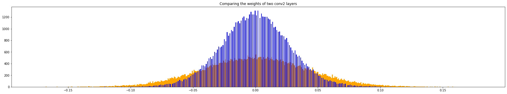
추가적으로 위 그림은 두번째 covolutional layer의 weight에 대한 분포이다.

knowledge distillation

나중에 추가…

이전Week08 Day36

다음Week08 Weekend